Machine Learning – Stanford -Week 8 – Clustering and PCA

Clustering – K-means algorithm

Continuing with Andrew Ng’s course and finally finished week 8 and delivered homework before deadline. So here again just to note some key points.

K-means

Basically speaking the K-means method is very simple and strait forward, one only need to repeat 1. assigning all samples to one of the closest centroids; 2. move centroids to the middle of those assigned samples. However the implementation is a little tricky to make correct due to the indexing.

And it is worth to mention that not only well separated clusters, but also a group of connected well (or non-separated clusters) can be also clustered via K-means method. This can be particularly useful, for example, a T-shirt company would like to only make S, M and L size of T-shirt for all people with different height and weight.

 

And here is a Pop-quiz:

---

 

More about random initialization

We could imagine that, when k is relatively small (for example k in range of 2 to 10), there is a big chance that the random initialization will put some centroids very close to each other in the beginning and result in some local optima.

The way to solve this issue is also very simple – do clustering (with random initialization) multiple times and then select the centroid group with the lowest cost.

---

 

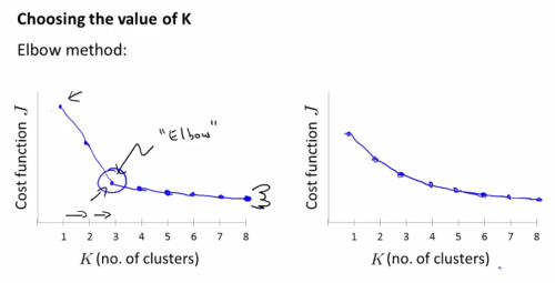
Choosing the value of K

Another question is how should we choose or decide how many clusters should there be for our data. Andrew suggested two method:

1. Elbow method, which is running the K from 1 to many and if we could see a clear “elbow” shape of cost curve, we can choose the K of that elbow point.
2. Based on practical or business/application specification.

---

 

Okay, so here are some pop quiz for K-means clustering:

---

 

And here I would like to add a image compression result made from the homework result – so for this example we used K-means clustering to cluster all pixels of a image with only 8 colors, and the original image is in RGB color of 256 colors. With K=8 we could use the algorithm to cluster all pixels with similar colors into one of the 8 colors. Notably that the value of the 8 colors are not pre-defined, they will gradually become some of the major colors on the picture (while the “moving centroids step” in the k-means algorithm). After the clustering is done, we can simply do the compression by finding the nearest centroid of every pixel and then assign that pixel of that color of centroid. Since we only have 8 colors, a 3 bit storage room for each pixel will be enough, while the 8 centroids are holding a RGB color each as the “cluster center” color 🙂

---

 

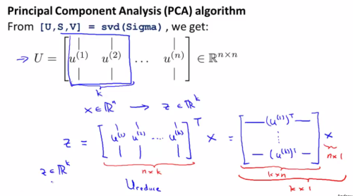
Principal Component Analysis – PCA

The motivation of principal component analysis is mainly about data compression – for example, how to casting a high dimension data down to a lower dimension space. This will help saving space of data storage, also improving certain algorithm speed, and also to help visualization since a data more than 3D, 4D will become impossible to be visualized directly.

So the so-called Principal Component Analysis (PCA) is just a method of reduce high dimension data to lower dimension data.

One thing we should notice is that even though it looks similar, but PCA and linear regression are two different algorithms and the goal is also totally not the same. For linear regress we have a value y we would like to predict, however for PCA all data are treated the same, there is no special label value.

PCA – How to

As Andrew mentioned, the mathematical proof of the following way of doing PCA is very difficult and also beyond the scope of the course, so here we just need to know how to use it instead. It turned out to just do a dimension reduction is actually very simple. Two lines of matlab code would be enough. The key is to utilize some build in “svd” function.

---

 

And a summary of the stuff above: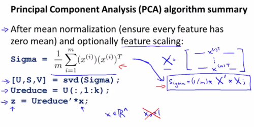

---

 

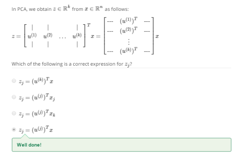
Again, here a pop quiz

---

 

Reconstruction

---

 

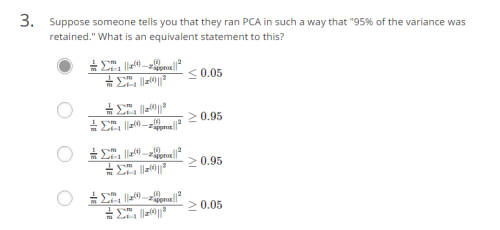
How to choose which level of dimension k we can reduce to?

Another quiz:

---

 

 

PCA – What can I use if for?

 

---

And some final pop quiz for under standing the topic better:

Machine Learning – Stanford -Week 5 – Neural Networks: Implementation

Continue with the Machine Learning course by Andrew Ng. This chapter we try to implement a simple Neural Network Classification algorithm.

Below is the definition of the problem.

 

Cost function 

Cost function is calculated as below.

Using the equation shown above, a sample MATLAB code calculating the cost function of a one layer Neural Network,  can be like this:

% First use forward propagation calculate the output h
a1 = [ones(m,1) X]; % m x 401
a2 = [ones(m,1) sigmoid(a1 * Theta1')]; % (m x 25) -> m x 26 
a3 = sigmoid(a2 * Theta2'); % (m x 26) * (26 x 10) = m by 10

% y is m by 10
h = a3;

for m_= 1:m
 a = 1:num_labels; % a is a temp para
 Y = (a == y(m_)); % classification label, 1 by 10 matrix
 J = J + ((-Y) * log(h(m_,:)') - (1-Y) * log(1-h(m_,:)')) ;
end

J = J/m;

% Plus regularization term
J = J + lambda/(2*m)* ( sum(sum(Theta1(:,2:end).^2)) ...
 + sum(sum(Theta2(:,2:end).^2)));

 

Gradient Computation

The following graphs are shown to illustrate the method of computing gradient.

Following the previous example code, here we can see am MATLAB implementation of a simple one layer Neural Network algorithm, with the part of code that calculate the gradient:

D1 = zeros(size(Theta1));
D2 = zeros(size(Theta2));

% Part 2 - back propagation
for t = 1:m

 % Step 1: perform forward propagation

 a1 = [1 X(t,:)]; % 1 x 401

 z2 = a1 * Theta1'; % 1x25
 a2 = [1 sigmoid(z2)]; % (1 x 25) -> 1 x 26 

 z3 = a2 * Theta2'; % (1 x 26) * (26 x 10) = 1 by 10
 a3 = sigmoid(z3) ;% 1x10

 % Step 2: using y to calculate delta_L

 a = 1:num_labels; % a is a temp para
 Y = (a == y(t)); % making Y matrix as classification label

 d3 = a3 - Y; % 1 by 10

 % Step 3: backward propagation to calculate delta_L-1,
% delta_L-2, ... until delta_2. (this example only have one layer,
% so only need to calculate delta_2)

 d2 = Theta2' * d3'; % 26 x 1
 d2 = d2(2:end); % 25 x 1
 d2 = d2 .* sigmoidGradient(z2)';

 % Alternatively:
 %d2 = Theta2' * d3' .* a2' .* (1-a2)'; % 26 x 1
 %d2 = d2(2:end); % 25 x 1

 % Step 4: accumulate Delta value for all m input data sample
 % Theta1 has size 25 x 401
 % Theta2 has size 10 x 26

 D2 = D2 + d3' * a2; % 10 x 26
 D1 = D1 + d2 * a1; % 25 x 401

end

% Finally, calculate the gradient for all theta
Theta1_grad = 1/m*D1 + lambda/m*[zeros(size(Theta1,1),1) Theta1(:, 2:end)];
Theta2_grad = 1/m*D2 + lambda/m*[zeros(size(Theta2,1),1) Theta2(:, 2:end)];
 

Some another illustrations to show how forward propagation and backward propagation are working. You might also want to use it to understand better on how to do the algorithm implementation.

A sample of how to use advanced optimization function to find the best Theta solutions (with some vector reshape operation needed):

Here is a pop quiz about it:

A short summary about the learning algorithm procedure.

 

Gradient Checking

Since the Neural Network algorithm is quite complicated and might be very buggy, so one good practice is that during implementation process, one can simultaneously calculate gradients by a numerical estimation method, and check if this value close enough to the gradient calculated by the learning algorithm.

This will help to generate the bug free code. And one should remember to turn the gradient checking function off when using the learning algorithm in production environment, since this numerical estimation method is very computational expensive.

 

Theta Initialization

Why do we have to use a random theta initialization?

 

Summary

 

End of the course. Pop quiz 

Congratulations, if you have followed the course so far, you will have a good understanding about Neural Network learning algorithms. If you also have done the course MATLAB exercise, you will be amazed by how “simple” it is that, just with a few lines of code, a learning algorithm can learn by itself to recognize hand written numbers.

I personally think Neural Network Learning is a very powerful tool and in the future it might have great potential to form very intelligent programs that can automatize lots of tedious works for people.

Thank you Andrew Ng for providing such a great course for everyone on the planet who is interested in machine learning. You are wonderful 🙂

Machine Learning – Stanford -Week 4 – Neural Networks: Representation

 

The following content from edX course Machine Learning taught by Andrew Ng.

Introduction to Neural Networks

Welcome to week 4! This week, we are covering neural networks. Neural networks is a model inspired by how the brain works. It was very widely used in 80s and early 90s; popularity diminished in late 90s (computationally expensive).

Recent resurgence: State-of-the-art technique for many applications. It is widely used today in many applications: when your phone interprets and understand your voice commands, it is likely that a neural network is helping to understand your speech; when you cash a check, the machines that automatically read the digits also use neural networks.

---

 

Why we need a new algorithm?

Feature “explosion” for logistic regression. Neural network will hopefully help solving this issue.

The “one learning algorithm” hypothesis

---

 

How it can solve complex non-linear problem

Key point

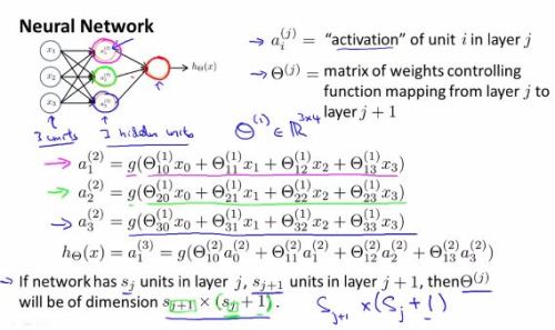
If network has units in layer j,  units in layer j+1, then will be of dimension

This is very important to know or memorize later on for doing vectorized implementation. Or see pop quiz below.

---

 

Non-linear classification example

---

 

Multiple output units: One-vs-all

---

 

Pop Quiz

 

Machine Learning – Stanford -Week 3 – Overfitting and Regularization

The following content is from Coursera Machine Learning course, taught by Andrwe Ng.

Overfitting

 

Regularization

 

Gradient descent with regularization

Regularization makes the matrix always invertable.

Pop Quiz

Spark Essentials

Quick notes on some basic info about Spark, materials from BerkeleyX: CS190.1x Scalable Machine Learning on edX.

Why we may want to use Spark:

Resilient Distributed Dataset (RDD)

• RDD cannot be changed after they are constructed
• They can be created by transformations applied to existing RDDs
• They enable parallel operations on collections of distributed data
• They track lineage information to enable efficient recomputation of lost data

 

Some basic Spark concept: Transformations

• Transformations are not computed right away
• Transformations are not vulnerable to machine failures
• Transformation are like a recipe for creating a result

 

Some basic Spark concept: Actions

Property of Spark Actions:

• They cause Spark to execute the recipe to transform the source data
• They are the primary mechanism for getting results out of Spark
• The results are returned to the driver

 

About Cashing RDD

If you plan to reuse an RDD, you should cache it, so that these RDD don’t have to be read again and again from hard-drive, instead they can be accessed from RAM.

 

Spark Programming Life-cycle

Some key points about Spark Program Lifecycle:

• RDDs that are reused may be cached
• Transformations lazily create new RDDs
• Transformations create recipes for peforming parallel computation on datasets
• Actions cause parallel computation to be immediately executed

 

A few words about Key-Value Transformations

 

PySpark Shared Variables:

In iterative or repeated computations, broadcast variables avoid the problem of repeatedly sending the same data to workers. Broadcast variables are an efficient way of sending data once that would otherwise be sent multiple times automatically in closures.

Accumulators can only be written by workers and read by the driver program.

Machine Learning – Stanford -Week 3 – Logistic Regression

Classification by regression

Great things learned again from Coursera Machine Learning course, taught by Andrwe Ng. Here are some of the key notes. Perhaps the first thing to notice here is that, even though the title of this article seems to be about regression, but it is actually a way of doing classification. So I think we could simply saying that “logistic regression” is a “classification” method.

How we got the idea?…(some background info)

If we follow from the previous linear regression course, we can naturally ask, can one use linear regression for Classification?

Answer is yes, like the simple example above where a hypothesis line is generated to do classification in a way that: if h larger than 0.5, predict class A, if h less than 0.5, predict class B.

However there are many limitations with this way. An apparent one is that when some cases appears, such as if a training sample appear on the far right of the graph (malignant tumor with very large size), the h function’s slop changes and will result in that some of other prediction to be wrong.

Logistic Function (or Sigmoid Function)

In order to solve this, we can shape the hypothesis function h as a logistic function, defined as follow, where the value of h can only change between 0 and 1.

Cost Function

When using logistic function as the hypothesis, we have to change the format of cost function a bit. Because for the previous way of defining cost function, the cost function will have many “local minimum” introduced because using logistic function. And this won’t help the gradient descent algorithm to work properly. 

Thus, we can defined the following cost function, so that is will be come “convex” and “gradient descent friendly”.

And, lucky or mathematically, the above cost function can be defined or re-written in the math format as following:

So by now, we have fully defined a simple classification problem and a group of classification hypothesis and cost function are ready to use.

Gradient Descent

And here is what the gradient descent algorithm looks like for Logistic Regression.

And here is a MATLAB version of the implementation of the algorithm above:

function [J, grad] = costFunction(theta, X, y)
%COSTFUNCTION Compute cost and gradient for logistic regression
% J = COSTFUNCTION(theta, X, y) computes the cost of using theta as the
% parameter for logistic regression and the gradient of the cost
% w.r.t. to the parameters.

% Initialize some useful values
m = length(y); % number of training examples
h=sigmoid(X*theta); % m by 1

J = 1/m * ((-y')*log(h) - (1-y')*log(1-h)); % 1 by 1

grad = 1/m * X'*(h-y); % n by 1, gradient

end

Hypothesis Interpretation

And a few more words (or pictures) discuss the interpretation of the hypothesis function output – basically speaking, it output a probability measure.

Decision Boundary

Continue the interpretation above, here we define the concept of “decision boundary” (which is a line for the case of 2 features):

And it can be non-linear, high order as well:

Multi-class Classification

So for the case of more than 2 classes, one can use the so called “one-vs-all” (or “one – vs-rest”) method to finish the job.

A few more words about some other optimization algorithm (such as fminunc in Qctave):

Machine Learning – Stanford -Week 2 – Linear Regression

Great knowledge learned from the Couresra course – Machine Learning (Stanford) taught by Andrew Ng. Here is a short summary of Week 2 ‘s content.

Gradient Descent

Perhaps the most important algorithm for linear regression. And it is also very intuitively understandable. Basically speaking the whole idea is similarly like you drop a ball on a sloped curve or surface (cost function) and ball roll down the surface following the gradient so that in the end the ball will be at the lowest point of the surface. The “surface” metaphor is used here for the situation that the cost function has two variables – sometimes called the weight. The “weight” parameters in the lecture represent by , and cost function is labeled as J.

So when the ball reaches the lowest point, the cost function J has the minimum value, which means if we use this group of weights to do prediction / regression, we get the best guess. And sometimes, for example in another Machine Learning course on Coursera (the one from University Washington), the cost function is referred as RSS – Residual Sum of Squares, which is more or less the same thing here as J.

The above cost function J can be calculated, for example in MATLAB code:

function J = computeCostMulti(X, y, theta)
%COMPUTECOSTMULTI Compute cost for linear regression with multiple variables
% J = COMPUTECOSTMULTI(X, y, theta) computes the cost of using theta as the
% parameter for linear regression to fit the data points in X and y

% Initialize some useful values
m = length(y); % number of training examples

J = 1/2/m * sum((X*theta-y).^2)

end

And the Gradient Descent algorithm is fairly simple, as described in the picture below, equation at upper right corner.

In MATLAB, it can be written a simple line of code, suppose X, y and theta are all in matrix format.

function [theta, J_history] = gradientDescentMulti(X, y, theta, alpha, num_iters)
%GRADIENTDESCENTMULTI Performs gradient descent to learn theta
% theta = GRADIENTDESCENTMULTI(x, y, theta, alpha, num_iters) updates theta by
% taking num_iters gradient steps with learning rate alpha

% Initialize some useful values
m = length(y); % number of training examples
J_history = zeros(num_iters, 1);

for iter = 1:num_iters

theta = theta - alpha/m*(X'*(X*theta - y));

% ============================================================
% Save the cost J in every iteration
J_history(iter) = computeCostMulti(X, y, theta);

end

end

Note that the sum in the equation is accomplished by matrix product operation in the code. Or, more precisely, if sample number is m and feature number is n then:

• X is m by n+1 matrix
• y is m by 1 matrix
• theta is n+1 by 1 matrix
• X*theta is m by 1 matrix
• X’ is n+1 by m matrix

Tips on how to choose (alpha) – Learning Rate

Basically, one can start with 0.001 and make it larger by 3 times each time until the cost function may not converge. Then you may end up finding a fast and also converging alpha.

Here is pop quiz for getting the idea of the effect of different value of learning rate (or step length):

Feature Scaling

It’s also very important to notice about feature scaling when using gradient decent algorithm, especially when there are multiple features and some of them have very different scales. If those features are not scale or normalized, the algorithms may now work efficiently.

One way to scale the features is called mean normalization, basically see pictures below.

Polynomial Regression

The powerful thing about gradient descent is that it is not just work for linear equations, it can be simple applied for any format of polynomial regression – one simply use higher orders of features as input features, illustrated below:

One thing worth mention is that feature scaling will become fairly important in order to make the polynomial regression work, since a high order of feature will be scaled very differently than the low order  feature.

Another Method – Normal Equation

One can also choose to not using gradient decent and instead use normal equation method (called closed form solution on course from University of Washington.

The basic idea is that by setting the derivative of cost function equals zero then directly solve the equation to get values of weight parameters. One thing worth mention is that for normal equation method, feature scaling is not needed at all. However mathematically this method has the complexity of O(n^3), where n stands for feature number. Thus for a problem has many features, one should probably choose gradient descent rather than this normal equation method. More discussion on this below.

Similar topic discussed in University of Washington course, with only two weight parameters – w0 and w1:

I didn’t verify but I guess the two equations from the two different lectures to calculate the weights by setting the derivative of cost function equals zero, are giving identical results, for the situation that the length of weight parameters are two.

Differences between Gradient Descent and Normal Equation

Or when to use Gradient Descent and when to use Normal Equation?

Answer is below:

Data Science and Machine Learning Essentials – Pop Quiz 1

The company Internet Movies, Inc. has found wide success in their streaming movie business. After many long and successful years of delivering content, they have decided to use machine learning to make their business even more successful. Luckily, they already possess a huge dataset that has grown over years and years of user activity – but they need your help to make sense of it! Answer the following questions

1. Let’s start with a simple case. Assume user Alice is a particularly good member and she makes sure to rate every movie she ever watches on the website. What machine learning approach would be better for the company to use for determining whether she would be interested in a new specific movie?

• Supervised
• Unsupervised

---

 

2. Bob, on the other hand, is not that much into ratings. He does watch a lot of movies, but never takes the time to rate them. For users like Bob, which of the following data can the company use to determine potential interest in a specific movie? Check all that apply.

• Metadata of movies: actors, director, genre,etc.
• Length of the movie
• Popularity of the movie among other users
• User login patterns

---

 

3. What machine learning approach should the company use for cases like Bob?

• Supervised
• Unsupervised

---

 

Now that the company has some idea about how to use the data, it’s time to design a classifier. Our classifier will be very simple: given a movie and a user, it will classify the movie as either “Good” or “Bad” for this user.

4. Assume all the users of the company have a very simple rule in their movie taste: they like it if Tom Cruise has the lead role. Any other data is mostly irrelevant. However, no one in the company knows about this fact. Which of the following clustering models might be able to detect this rule? Check all that apply.

• Supervised (label: rating), with data: Director, language, genre
• Supervised (label: rating), with data: Movie length, lead role, director
• Unsupervised, with data: Lead role, genre, director
• Unsupervised, with data: Number of ratings, lead role

---

 

5. Looking at the options they’re given, the board members choose to go with a supervised model with lead role as data. You become outraged. “How can you not include movie length? It’s incredibly important! Who watches a 3 hour long movie –” Your fellow data scientist interrupts you. “Yeah, I agree, but look at these initial results. You see, if we remove movie length, …” What can your colleague (correctly) say to convince you? Check all that apply.

• “we can reduce inter-cluster dissimilarity.”
• “we can reduce intra-cluster dissimilarity.”
• “the model starts to work. It doesn’t work otherwise.”
• “we can consume less memory, and the results look almost the same.”

---

---

Answer:

1. Supervised

2. Choose:

• Metadata of movies: actors, director, genre, etc.
• Popularity of the movie among other users

Explanation:Length of the movie may or may not be considered. We are more likely to consider it if we consider very long movies or very short movies as well.

3. Unsupervised

4. Choose:

• Supervised (label: rating), with data: Movie length, lead role, director
• Unsupervised, with data: Lead role, movie length, rating

Explanation: For supervised learning, we already have ratings for each label. So for the data to differentiate between those with Tom Cruise or not, we must have the leading role as one of our features. For unsupervised learning, we must have the lead role as part of our data. In addition, we must have a way to know whether users like the movie or not, so we must also know the rating.

5. Choose:

• “we can reduce intra-cluster dissimilarity.”
• “we can consume less memory, and the results look almost the same.”

Explanation: Movie lengths are not sufficiently different between most movies in order to help us in making the clusters. Reducing intra-cluster dissimilarity is correct because having less features allows us to differentiate elements within a cluster from each other. Consuming less memory with similar results is correct because we do not need as much storage and will save money. The supervised learning model will work and has no limits on the number of features allowed.

---

Note: above content is from edX.

 

Data Science and Machine Learning Essentials – Module1- Clustering

Clustering

• Clustering groups data entities based on their feature values. Each data entity is described as a vector of one or more numeric features (x), which can be used to plot the entity as a specific point.

• K-Means clustering is a technique in which the algorithm groups the data entities into a specified number of clusters (k). To begin, the algorithm selects k random centroid points, and assigns each data entity to a cluster based on the shortest distance to a centroid. Each centroid is then moved to the central point (i.e. the mean) of its cluster, and the distances between the data entities and the new centroids are evaluated, with entities reassigned to another cluster if it is closer. This process continues until every data entity is closer to the mean centroid of its cluster than to the centroid of any other cluster. The following image shows the result of K=Means clustering with a k value of 3:

• Hierarchical Agglomerative Clustering is an alternative clustering technique in which the point representing each data entity begins as its own cluster. Each cluster is then merged with the cluster closest to it, and this merging process continues iteratively. The following image illustrates the process of Hierarchical Agglomerative Clustering.

• The distance metric used to determine how “close” points are to one another is an important aspect of clustering. The simplest way to conceptualize the entities is as points in Euclidean space (multidimensional coordinates), and measure the simple distance between the points; but other distance metrics can also be used.
  

Data Science and Machine Learning Essentials – Module1- Classification

Classification and Loss Function

• For a classification function to work accurately, when operating on the data in the training and test datasets, the number of times that the sign of f(x) does not equal y must be minimized. In other words, for a single entity, if y is positive, f(x) should be positive; and if y is negative, f(x) should be negative. Formally, we need to minimize cases where y ≠ sign(f(x)) to let the classification function to work accurately.
• Because same-signed numbers when multiplied together always produce a positive, and numbers of different signs multiplied together always produce a negative, we can simplify our goal to minimize cases where yf(x) < 0; or for the whole data set ∑_iy_if(x_i) < 0. This general approach is known as a loss function.
• As with regression algorithms, some classification algorithms add a regularization term to avoid over-fitting so that the function achieves a balance of accuracy and simplicity (Occam’s Razor again).
• Each classification algorithm (for example AdaBoost, Support Vector Machines, and Logistic Regression) uses a specific loss function implementation, and it’s this that distinguishes classification algorithms from one another.

Decision Trees and Multi-Class Classification

• Decision Trees are classification algorithms that define a sequence of branches. At each branch intersection, the feature value (x) is compared to a specific function, and the result determines which branch the algorithm follows. All branches eventually lead to a predicted value (-1 or +1). Most decision trees algorithms have been around for a while, and many produce low accuracy. However, boosted decision trees (AdaBoost applied to a decision tree) can be very effective.
• You can use a “one vs. all” technique to extend binary classification (which predicts a Boolean value) so that it can be used in multi-class classification. This approach involves applying multiple binary classifications (for example, “is this a chair?”, “is this a bird?”, and so on) and reviewing the results produced by f(x) for each test. Since f(x) produces a numeric result, the predicted value is a measure of confidence in the prediction (so for example, a high positive result for “is this a chair?” combined with a low positive result for “is this a bird?” and a high negative result for “is this an elephant?” indicates a high degree of confidence that the object is more likely to be a chair than a bird, and very unlikely to be an elephant.)

Imbalanced Data

• When the training data is imbalanced (so a high proportion of the data has the same True/False value for y) , the accuracy of the classification algorithm can be compromised. To overcome this problem, you can “over-sample” or “weight” data with the minority y value to balance the algorithm.

ROC – Receiver Operator Characteristic

• The quality of a classification model can be assessed by plotting the True Positive Rate (predicted positives / actual positives) against the False Positive Rate (predicted negatives / actual negatives) for various parameter values on a chart to create a receiver operator characteristic (ROC) curve. The quality of the model is reflected in the area under the curve (AOC). The larger this area is than the area under a straight diagonal line (representing a 50% accuracy rate that can be achieved purely by guessing), the better the model; as shown below: